
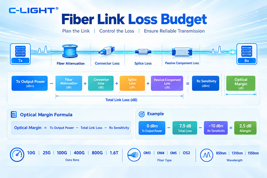
Fiber link loss budget is the calculation used to determine whether an optical link has enough power margin for reliable transmission. It accounts for fiber attenuation, connector loss, splice loss, optical components, transceiver power, receiver sensitivity, and engineering margin across 10G, 25G, 100G, 400G, 800G, and higher-speed networks.
A fiber link loss budget defines the maximum optical loss that a fiber link can tolerate while still meeting the receiver's required operating conditions.
It compares the optical power available from the transmitter with the minimum optical power required by the receiver after accounting for all losses in the optical path.
A fiber link can fail even when the fiber itself is functional if the total optical loss is higher than the available system budget.
Loss-budget analysis helps determine whether a planned optical path will support the selected transceiver before the network is installed.
A simplified optical loss budget can be represented as:
Link Loss Budget = Minimum Transmitter Output Power − Receiver Sensitivity
The remaining margin is then reduced by actual fiber attenuation, connector loss, splice loss, and other optical penalties.
A practical calculation can be written as:
Optical Margin = Tx Output Power − Total Link Loss − Rx Sensitivity
A positive margin indicates that the calculated received power remains above the receiver sensitivity under the defined conditions.
Fiber attenuation: Optical loss along the fiber length.
Connector loss: Loss introduced by mated optical connectors.
Splice loss: Loss caused by fusion or mechanical splicing.
Passive component loss: Loss from splitters, WDM devices, adapters, and other components.
Transceiver limits: Transmitter output and receiver sensitivity.
Engineering margin: Additional allowance for real-world variation.
Fiber attenuation is the optical power lost as light travels through the fiber. It depends on fiber type, wavelength, length, and installation conditions.
Loss is normally expressed in dB/km or dB/m depending on the application.
Each optical connector introduces some insertion loss. A link with many patch points can therefore consume significantly more optical budget than a direct point-to-point connection.
Splices create additional optical loss. Although a properly executed fusion splice can have relatively low loss, multiple splices can accumulate significant total loss in a long optical route.
Optical links can include additional passive components such as WDM multiplexers, demultiplexers, adapters, patch panels, splitters, and optical switches.
Each component must be included in the total loss calculation.
Receiver sensitivity is the minimum optical input power required to achieve the specified performance under a defined test condition.
A more sensitive receiver generally provides greater tolerance to optical loss, assuming the rest of the link remains within specification.
Transmitter output power defines the amount of optical power launched into the fiber. The actual minimum and maximum values should be taken from the transceiver specification rather than using a nominal value alone.
For conservative loss-budget calculations, the minimum specified transmitter power is normally more useful because it represents a worst-case available optical input to the link.
Using only the typical transmit power can overestimate the available margin.
The receiver sensitivity value used for system design should correspond to the applicable specification and test condition. Different modulation formats, wavelengths, data rates, and receiver architectures can have different sensitivity values.
Total link loss is the sum of all relevant losses in the optical path:
Total Link Loss = Fiber Loss + Connector Loss + Splice Loss + Passive Component Loss
Additional penalties should be included where required by the specific optical system.
Fiber loss can be estimated with:
Fiber Loss = Fiber Length × Fiber Attenuation
For example, a 10km fiber with an assumed attenuation of 0.4dB/km would contribute 4dB of fiber loss before connectors, splices, and other components are added.
If a link has four mated connector pairs and each pair contributes 0.3dB, the total connector loss would be:
4 × 0.3dB = 1.2dB
If six splices each contribute 0.1dB, the total splice loss would be:
6 × 0.1dB = 0.6dB
Consider a simplified optical link with:
Minimum Tx power: 0dBm
Fiber loss: 5dB
Connector loss: 1.2dB
Splice loss: 0.6dB
Other passive loss: 0.7dB
Receiver sensitivity: -10dBm
The total link loss is:
5 + 1.2 + 0.6 + 0.7 = 7.5dB
The estimated received power is:
0dBm − 7.5dB = -7.5dBm
The remaining optical margin is:
-7.5dBm − (-10dBm) = 2.5dB
A link should not normally be designed to operate exactly at the calculated sensitivity limit. Fiber aging, connector contamination, temperature, repairs, manufacturing variation, and future network changes can reduce the available margin.
The required engineering margin depends on the application and network design. A margin of several dB may be used in many practical designs, but the appropriate value should come from the applicable engineering rules and system requirements rather than a universal fixed number.
These terms are closely related but can be used differently. Optical power budget describes the power difference available between transmitter and receiver limits, while link loss budget focuses on how much loss the physical optical path can accommodate.
| Term | Meaning |
|---|---|
| Power budget | Available optical power difference between transmitter and receiver limits |
| Link loss budget | Maximum allowable physical link loss |
| Link margin | Remaining performance margin after actual losses |
Multimode links are commonly used for short-reach data center applications. The loss budget depends on the fiber type, wavelength, connector count, length, transceiver, and network speed.
Single-mode fiber is widely used for longer data center, campus, metro, and DCI links. As the physical distance increases, fiber attenuation becomes a larger part of the total loss budget.
OM3 is commonly used for short-reach 850nm data center applications. The allowable channel loss depends on the specific transceiver and standard.
OM4 provides higher modal bandwidth than OM3 and is widely used for high-speed short-reach optical links.
The loss budget still needs to be calculated using the exact module and installed channel.
OM5 is designed for wideband multimode applications and can support certain wavelength-multiplexed architectures. The loss budget depends on the wavelength range and specific optical system.
OS2 single-mode fiber is widely used for longer high-speed links. Its low attenuation makes it suitable for data center backbone, campus, metro, and DCI applications.
Fiber attenuation varies with wavelength. A loss-budget calculation should therefore use attenuation values corresponding to the optical wavelength used by the transceiver.
850nm is commonly used for VCSEL-based multimode data center applications. The fiber loss and transceiver specifications should be evaluated together when calculating the usable reach.
1310nm is widely used in single-mode optical transceivers such as LR, DR, FR, and ER-related architectures.
The lower fiber attenuation and different dispersion characteristics at this wavelength make it suitable for longer transmission.
1550nm is important for longer-distance optical communication because fiber attenuation is relatively low and optical amplification technologies are well established around this wavelength.
10G optical links can use multimode or single-mode fiber depending on the application. Short-reach SR links generally have lower channel-loss requirements, while LR and extended-reach solutions require a carefully calculated power budget.
25G optical systems use several transceiver types with different reach and optical power characteristics. The exact loss budget should be calculated from the selected module's transmitter and receiver specifications.
100G transceivers can use architectures such as SR4, DR, LR4, ER4, and other variants. Each architecture has different optical power, sensitivity, wavelength, and reach characteristics.
100G ER4 is a long-reach four-wavelength architecture and is particularly sensitive to total link loss. The C-LIGHT CL100GQSFPER4 specification provides a maximum transmitter and dispersion penalty of 2.5dB and an OMA receiver sensitivity of up to -21.4dBm per lane.
Its 40km capability must be evaluated as an engineered optical link rather than assuming that every 40km fiber route will automatically operate without additional loss analysis.
400G optical architectures can include SR, DR, FR, LR, and other designs. The loss budget varies significantly between multimode parallel optics and single-mode WDM or parallel-optics solutions.
800G increases the importance of accurate channel-loss calculations because higher-speed PAM4 signals operate with tighter optical and electrical margins.
Transceiver type, wavelength architecture, connector count, and fiber type can all materially change the available system margin.
1.6T optical architectures introduce even tighter signal-quality requirements. Depending on the implementation, the system may use multiple wavelengths, parallel single-mode fibers, or other optical configurations.
PAM4 systems are more sensitive to signal quality than conventional binary NRZ architectures. Optical power alone is therefore not always enough to describe the complete link margin.
OMA, TDECQ, receiver sensitivity, BER, and FEC behavior may also need to be considered.
NRZ uses two primary signal levels and is generally simpler to characterize than PAM4. Nevertheless, the physical link still needs sufficient optical power and signal quality to meet the required BER.
WDM systems use multiple wavelengths over the same fiber. Multiplexers and demultiplexers introduce additional insertion loss that must be included in the link budget.
CWDM systems typically use wider wavelength spacing and are commonly deployed in access, metro, and enterprise networks. The MUX/DEMUX loss should be included alongside fiber and connector losses.
DWDM systems can contain multiple wavelengths, filters, multiplexers, demultiplexers, ROADMs, and amplifiers. The complete optical path can therefore be considerably more complex than a simple point-to-point fiber link.
When a WDM component is inserted into the link, its specified insertion loss must be included separately for the relevant wavelength.
ROADM systems add optical switching and filtering functions to the transmission path. Each node can consume part of the available optical budget.
Optical amplifiers can compensate for accumulated optical loss, but they also introduce noise. A long-distance optical system must therefore consider both optical power and OSNR.
Data Center Interconnect links can contain long fiber spans and multiple passive or active optical components. A DCI loss budget should therefore account for the entire route, including patching, WDM equipment, amplification, and ROADMs where applicable.
Coherent pluggables use advanced DSP and coherent detection to tolerate demanding optical conditions. Their link engineering typically considers not only power but also OSNR, dispersion, nonlinear effects, and the characteristics of the optical line system.
Increasing transmit power can improve received power, but excessive optical power can increase nonlinear penalties in some DWDM systems. Therefore, long-distance coherent links must balance launch power against OSNR and nonlinear effects.
Connector count can have a substantial impact on short and medium links. A design with many patch points can consume a large fraction of the available optical budget even when fiber attenuation is low.
MPO connections can simplify multi-fiber cabling but require careful loss planning. Every MPO connector pair, cassette, adapter, and breakout assembly can contribute to total insertion loss.
MPO-12 systems are widely used for high-density parallel optical links. The actual loss must be taken from the connector and cabling specifications used in the installed system.
MPO-16 can provide higher fiber density for applications such as some 800G and next-generation optical architectures. The connector loss and fiber mapping should be included in the optical budget.
LC connectors are widely used for duplex and WDM optical modules. Although each connector pair can have low insertion loss, multiple LC connection points can accumulate measurable loss.
Patch panels introduce additional connection points and may include adapters, cassettes, or splice functions. These losses should be included in the complete link calculation.
Fiber cassettes can simplify structured cabling but add another passive optical interface. The manufacturer's specified insertion loss should be included in the link budget.
Incorrect polarity does not normally create a conventional insertion-loss problem; instead, it connects the wrong transmit and receive fibers and can prevent the link from operating.
Polarity should therefore be verified separately from optical loss.
Insertion loss describes how much optical power is lost through a component, while return loss describes how much optical power is reflected toward the source.
Both can affect system performance but they represent different optical characteristics.
Excessive reflections can affect transmitters, receivers, and sensitive high-speed optical systems. Return-loss specifications should therefore be checked when designing demanding optical links.
Sharp bends can increase attenuation, particularly when cable routing exceeds the specified minimum bend radius.
Proper routing and cable management help prevent unexpected loss after installation.
Environmental conditions can influence fiber and component behavior. Optical transceiver specifications should be checked across the required temperature range when designing a critical link.
Long-term operation can introduce additional variation through connector contamination, fiber repairs, equipment replacement, and component aging.
An engineering margin provides tolerance for these changes.
Contamination can produce unexpectedly high insertion loss and reflection. This is one of the first items to check when a measured link loss is significantly higher than the calculated value.
Connectors should be cleaned and inspected before loss measurements. Testing a contaminated connector can produce a misleadingly high loss result and may also contaminate the mating connector.
An optical loss test set can measure the end-to-end insertion loss of a fiber channel. The measured value can then be compared with the calculated loss budget.
Optical loss measurements depend on the selected reference method and test configuration. Reference cords, adapters, connector interfaces, and instrument calibration can all influence the result.
OTDR testing can identify the location of abnormal loss events, splices, connectors, and reflections along a fiber route.
OTDR results can complement end-to-end insertion-loss measurements but should not automatically be treated as equivalent measurements.
Calculated loss predicts expected performance based on component specifications. Measured loss verifies the installed physical channel.
Both are useful because a link can meet a theoretical budget but fail to meet expectations if installation quality introduces additional loss.
A practical process is:
1. Identify the transceiver → 2. Record minimum Tx power → 3. Record Rx sensitivity → 4. Measure fiber length → 5. Determine fiber attenuation → 6. Count connectors → 7. Count splices → 8. Add passive component losses → 9. Add engineering margin → 10. Compare calculated and measured loss
| Loss Component | Example Loss |
|---|---|
| Fiber attenuation | 3.0dB |
| 4 connector pairs | 1.2dB |
| 2 splices | 0.2dB |
| Passive components | 0.5dB |
| Total calculated loss | 4.9dB |
Breakout architectures can introduce additional connector and branch losses. The complete optical path should be evaluated from the transmitting port to each receiving port.
An AOC contains integrated optical transceivers and fiber inside a fixed cable assembly. The user generally does not calculate individual fiber connectors inside the assembly, but the AOC's specified optical performance still needs to match the host system.
For separate optical transceiver and structured-fiber installations, the fiber plant and transceiver should be analyzed as a complete link.
AI data centers increasingly deploy 400G and higher-speed links. These systems can have tighter optical margins than traditional lower-speed networks, making accurate connector loss, fiber loss, and polarity control more important.
800G networks can use multi-lane PAM4 architectures and high-density MPO or WDM connectivity. The optical loss budget must match the exact transceiver architecture.
1.6T introduces even higher signaling rates and tighter system requirements. Accurate fiber qualification, connector control, and loss-budget planning are essential as port speeds increase.
Module selection should begin with the required distance and actual optical path. A module with a nominal reach longer than the intended link may still be unsuitable if the complete optical path introduces excessive loss or other penalties.
Compare the module's minimum transmitter power and receiver sensitivity with the calculated channel loss. Select a module that provides sufficient margin for the actual installation and expected operating variation.
A fiber link that works for 100G does not automatically provide sufficient performance for 400G or 800G. Higher-speed transceivers may have tighter optical and signal-quality requirements.
Future upgrades should therefore be considered during the initial cabling design.
High-quality low-loss connectors, adequate fiber type, correct polarity, sufficient patch-panel capacity, and appropriate cable routing can make future upgrades easier.
Backbone paths can contain longer fiber lengths and more cross-connects than equipment-side links. The resulting optical budget should include every passive component between network endpoints.
Campus links can span buildings and may contain outdoor fiber, patch panels, splice closures, and longer routes. Fiber attenuation and splice loss become more significant than in short data center connections.
Metro networks can contain multiple optical nodes, WDM equipment, amplifiers, and ROADMs. The optical budget becomes a system-level calculation rather than a simple fiber-length calculation.
DCI links require careful analysis of fiber span loss, connector count, WDM equipment, amplification, OSNR, and coherent module performance.
Using typical Tx power instead of minimum specified power.
Ignoring connector or splice loss.
Ignoring WDM or passive component insertion loss.
Using the wrong fiber attenuation value.
Assuming nominal transceiver reach guarantees field performance.
Ignoring engineering margin.
Using measured values without validating instrument references.
A transceiver labeled 10km, 20km, 40km, or another distance does not mean every fiber route of that length will operate under every installation condition.
Reach specifications are based on defined optical and system conditions and should be evaluated together with the actual link budget.
A long fiber route with only two connector pairs can have less total loss than a shorter route with many patch points. Connector count should therefore be included explicitly in the calculation.
Operating directly at the theoretical loss limit leaves little tolerance for real-world variation. An adequate engineering margin is important for stable long-term operation.
When a link exceeds the expected loss budget, start by checking connector cleanliness and insertion loss. Then inspect patch cords, adapters, splices, bends, fiber sections, and passive optical components.
If the fiber itself tests normally but the complete channel shows excessive loss, the problem may be located at connectors, patch panels, cassettes, adapters, or other interfaces.
If the calculated budget looks adequate but the link still fails, investigate wavelength, polarity, transceiver compatibility, receiver sensitivity, optical signal quality, electrical conditions, and measurement accuracy.
Use conservative transceiver specifications, calculate every passive loss, maintain an engineering margin, measure the installed channel, verify polarity, clean connectors, document every fiber path, and repeat the calculation whenever the optical topology changes.
| Parameter | Check |
|---|---|
| Transmitter | Minimum specified Tx power |
| Receiver | Required sensitivity |
| Fiber | Type, length, wavelength, attenuation |
| Connectors | Count and insertion loss |
| Splices | Count and measured loss |
| Passive components | MUX/DEMUX, splitter, adapter, cassette, ROADM |
| Margin | Adequate engineering margin |
| Testing | Measured end-to-end loss |
Fiber link loss budget is a fundamental part of optical network design. It determines whether the selected transceiver has sufficient optical power to overcome fiber attenuation, connector loss, splice loss, passive component loss, and other link penalties while maintaining adequate operating margin.
For modern networks from 10G to 400G, 800G, 1.6T, and beyond, loss-budget analysis is becoming increasingly important as optical margins tighten and network architectures become more complex.
The most reliable approach is to combine a conservative theoretical calculation with measured end-to-end loss. By accounting for every component in the optical path, maintaining an appropriate engineering margin, and validating the installed fiber infrastructure, network operators can reduce link failures and improve the reliability of high-speed optical networks.
For any questions, please contact us by email or WhatsApp.
Email: sales@c-light.com
WhatsApp: +86 132 6656 7067